


Google Sheets can turn a plain column of numbers into a chart in under a minute, but the difference between a chart that gets ignored and one that actually communicates something usually comes down to a few small decisions: which chart type fits the data, how it’s labeled, and whether it’s cleaned up enough to hand to someone else.
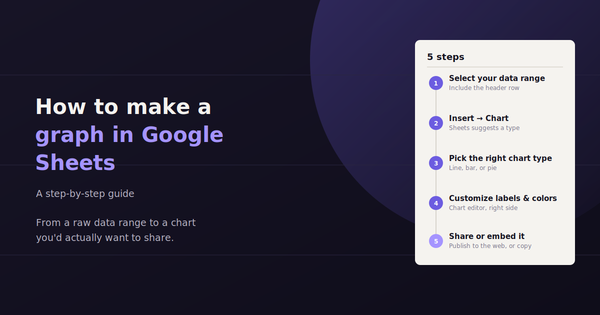
This guide walks through the full process — selecting your data, inserting a chart, choosing between line, bar, and pie charts, and customizing the result so it looks intentional rather than default. It’s written for anyone building a chart for a report, a client deck, or a team update, not just for spreadsheet power users.
Every step below uses Google Sheets’ built-in chart tools, so there’s nothing extra to install or connect.
Step 1: Organize and Select Your Data
Google Sheets reads chart data most reliably when it’s arranged in a simple table with headers in the first row and each category or time period in its own row. Clean structure upfront prevents most chart-building headaches later.
Before inserting anything, make sure your data is arranged in a way Google Sheets can interpret automatically. The most reliable layout is a simple table: one header row describing each column, and one row per data point below it.
For a chart tracking values over time — say, monthly revenue — put the time period (months, weeks, dates) in the first column and the metric in the second. For a chart comparing categories, like traffic by channel, put the category names in the first column and the values in the second.
Put column headers in row 1 — Google Sheets uses these as chart labels and legend text automatically.
Keep one variable per column; avoid merged cells within the data range, which can confuse the chart tool.
Remove blank rows or stray totals inside the range you plan to chart, since Sheets will try to plot them too.
Highlight the full range, including headers, by clicking and dragging, or by holding Ctrl (Cmd on Mac) to select non-adjacent columns.
Step 2: Insert the Chart
With your data selected, go to the Insert menu and choose Chart. Google Sheets will automatically generate a chart based on your selection and open the Chart Editor panel on the right side of the screen.
In most cases, Sheets makes a reasonable first guess at chart type based on your data shape — a line chart for data with a time-based column, or a column chart for categorical comparisons. That guess is a starting point, not a final answer, and it’s worth checking against the chart type guidance in the next section.
If the chart lands somewhere inconvenient, you can click and drag it by its edge to reposition it anywhere on the sheet, or resize it by dragging a corner handle.
Step 3: Choose the Right Chart Type
Line charts show trends over time, bar or column charts compare discrete categories, and pie charts show how parts make up a whole. Picking the wrong type is the most common reason a chart confuses rather than clarifies.
In the Chart Editor’s Setup tab, the Chart type dropdown lets you switch between every chart Sheets supports. The right choice depends entirely on what question the chart needs to answer, not personal preference.
| Chart Type | Best For | Avoid When |
|---|---|---|
| Line chart | Showing trends over time (traffic, revenue, rankings by week or month) | Comparing unrelated categories with no time dimension |
| Bar / Column chart | Comparing values across discrete categories (channels, products, regions) | You have more than 10–12 categories, which gets cluttered |
| Pie chart | Showing how parts make up a whole, with 6 or fewer segments | Comparing precise values — pie charts make small differences hard to read |
| Stacked bar chart | Comparing category totals while also showing their sub-components | The sub-components aren’t meaningfully related to each other |
| Scatter chart | Showing the relationship or correlation between two numeric variables | One of your variables isn’t actually numeric or continuous |
Step 4: Customize the Chart
Once the chart type is set, the Customize tab in the Chart Editor is where a generic default chart becomes something worth presenting. Every major visual element — title, axis labels, colors, legend position, and fonts — can be adjusted here without touching the underlying data.
Start with the basics that affect readability most: a clear chart title, labeled axes, and a legend position that doesn’t crowd the plotted data. From there, color and font choices are mostly about matching whatever deck, report, or brand style the chart needs to fit into.
Chart and Axis Titles
Under Chart & axis titles, add a clear, specific chart title rather than leaving the default blank or generic label. A title like “Monthly Organic Traffic, Jan–Jun 2026” tells a viewer what they’re looking at before they even read the axes.
Colors and Series Styling
The Series section lets you set a specific color for each data series, which matters most when a chart will be viewed alongside other charts that should share a consistent palette. Avoid Sheets’ full-saturation defaults for anything presentation-facing — slightly muted colors tend to read as more professional.
Legend and Gridlines
The Legend section controls where labels for each series appear; bottom or right placement usually keeps the chart itself uncluttered. Under Gridlines and ticks, reducing gridline density or removing minor gridlines entirely often makes a chart easier to scan at a glance.
Step 5: Make the Chart Presentation-Ready
A chart built for internal use and one built for a client or executive audience need different levels of polish: consistent colors, a specific and readable title, appropriate sizing, and no unnecessary gridlines or clutter.
A chart that’s technically correct isn’t automatically ready to show someone else. A few finishing touches make the difference between a chart that looks like a rough draft and one that looks intentional.
Use a specific title, not a generic one — “Q2 Ad Spend by Channel” reads better than “Chart 1.”
Round decimal values in data labels; three decimal places rarely add useful information to a presentation chart.
Keep colors consistent across every chart in the same report so a viewer doesn’t have to relearn what each color means.
Resize the chart to fill its intended space cleanly rather than leaving it at Sheets’ default dimensions.
If pasting into Slides or Docs, use Copy chart then Paste, and choose “Link to spreadsheet” so the chart updates automatically if the source data changes.
Working With Multiple Data Series
Charting more than one metric at once — like sessions and conversions on the same timeline — works well in Google Sheets as long as the series share a comparable scale, or a secondary axis is used when they don’t.
Many reporting charts need to show more than one metric at a time, like traffic alongside conversions, or spend alongside ROAS. Google Sheets handles this by simply selecting multiple value columns before inserting the chart — each becomes its own series, plotted together automatically.
The catch is scale. If one series ranges from 0 to 10,000 and another from 0 to 5, the smaller series will look flat and unreadable next to the larger one on a shared axis.
Using a Secondary Axis
When two series have very different scales, the Chart Editor’s Setup tab lets you assign one series to the right-hand axis instead of the left. Click the series in question, and under its axis setting choose the right axis, which gives each metric its own scale while still sharing the same chart.
Combo Charts
For cases like spend (a bar) plotted against a rate metric like ROAS (a line), a combo chart — available in the chart type dropdown — lets one series render as columns and another as a line on the same chart. This is a common pattern in marketing reporting, since it shows volume and efficiency together without needing two separate charts.
Building a Chart From a Pivot Table
For larger datasets — raw campaign-level exports, for example — building a chart directly from unsummarized rows often produces a cluttered, hard-to-read result. In these cases, it’s usually better to summarize the data in a pivot table first, then chart the pivot table’s output.
To do this, select your raw data range, go to Insert > Pivot table, and configure it to group and summarize the metric you want to chart (for example, total spend by campaign, or sessions by week). Once the pivot table is built, select its output range and insert a chart the same way as with any other data — the chart will reflect the summarized totals rather than every individual row.
Common Mistakes to Avoid
A handful of mistakes account for most confusing or misleading charts built in Sheets. Most are easy to catch with a quick second look before sharing.
The most frequent issue is choosing a chart type that doesn’t match the underlying question — a pie chart with twelve slices, or a line chart connecting categories that have no real order. The second most common issue is skipping axis labels or units entirely, which leaves a viewer guessing whether a number represents dollars, percentages, or raw counts.
Using a pie chart with too many segments, making it impossible to compare slices accurately.
Leaving axis labels blank, so a viewer can’t tell what unit the numbers represent.
Truncating the Y-axis in a way that visually exaggerates small differences — Sheets sometimes does this by default.
Charting a data range that includes a totals row, which distorts the scale of every other value.
When a Static Chart Isn’t Enough
A Google Sheets chart is a great fit for a one-off analysis, a single client report, or a chart embedded in a deck. It gets less practical as a recurring reporting solution, though, once you’re rebuilding the same chart every week across multiple data sources or multiple clients, since the underlying data has to be manually refreshed or re-pulled each time.
For that recurring use case, some teams move to a dedicated dashboarding tool, while others use a conversational reporting tool like ConvoData, which connects directly to live marketing data sources and answers plain-English questions on demand — skipping the manual chart-rebuilding step entirely for recurring reporting needs.
If you are setting up your broader Google presence, our guide to Google Brand Accounts and why your business needs one covers a commonly overlooked setup step. And once your data is chart-ready, our guide to building web analytics reports covers how to turn a one-off graph into a recurring report.
Frequently Asked Questions
How do I make a graph in Google Sheets from scratch?
Select your data including headers, go to Insert > Chart, then use the Chart Editor's Setup and Customize tabs to pick the right chart type and adjust titles, colors, and labels.
What's the difference between a line chart and a bar chart in Google Sheets?
Line charts are best for showing trends over a continuous period, like traffic or revenue by month. Bar or column charts are best for comparing discrete categories side by side, like performance across different channels.
Can I update a Google Sheets chart automatically when the data changes?
Yes — charts in Sheets update automatically whenever the underlying data range changes, and a chart copied into Google Slides or Docs with the 'link to spreadsheet' option will also update when you choose to refresh it.
How do I change the colors of a chart in Google Sheets?
Open the Chart Editor, go to the Customize tab, and use the Series section to set a specific color for each data series individually.
Why does my Google Sheets chart look wrong or empty?
This usually happens when the selected data range includes blank rows, merged cells, or a totals row, or when headers weren't included in the selection. Reselect a clean, header-included range and re-insert the chart.
What chart type should I use to show data over time?
A line chart is generally the best choice for time-based data like monthly traffic or weekly revenue, since it makes trends and direction easy to see at a glance.
How do I chart two metrics with very different scales on the same graph?
Assign one metric to a secondary (right-hand) axis in the Chart Editor's Setup tab, or use a combo chart so one metric renders as bars and the other as a line, each with its own scale.
Should I chart raw data or a pivot table summary?
For large, row-level datasets, building a pivot table first and charting its summarized output usually produces a cleaner, more readable chart than plotting every raw row directly.
If you’re building the same Google Sheets charts every week for client reporting, see how ConvoData turns that recurring chart-building work into a quick question you can ask in plain English.